One-sentence Summary

University of Cambridge and ETH Zürich propose a difference-in-differences method from econometrics that efficiently estimates per-instance memorisation profiles in language models by observing a small set of instances throughout training, with experiments on the Pythia suite revealing that memorisation is stronger in larger models, governed by data order and learning rate, and predictable across model sizes.

Key Contributions

• An unbiased and computationally efficient estimator for instance-level counterfactual memorisation is developed using a difference-in-differences design from econometrics, estimating how including a training instance changes a specific model's ability to predict that instance.

• A method for characterising a model's memorisation profile across training is proposed by observing a small set of instances throughout training, separating checkpoint timing, data order, and learning rate effects from architecture-level averages.

• Experiments with the Pythia model suite show that memorisation is stronger and more persistent in larger models, determined by data order and learning rate, and stable across model sizes, making memorisation in larger models predictable from smaller ones.

Introduction

Large language models are trained on web-scale corpora, yet they can reproduce training sequences verbatim, which matters for copyright, privacy, factual understanding, and training dynamics. Prior work defines memorisation causally, but measuring it is difficult because the counterfactual outcome, a model’s performance without training on an instance, is unobservable. Earlier estimates either require multiple training runs and therefore describe model architectures rather than specific models, or assume the counterfactual is negligible and may conflate memorisation with ordinary predictability. The authors leverage potential outcomes and econometrics to formalise counterfactual memorisation and propose an observational estimator based on training checkpoints and loglikelihood measurements. This yields memorisation profiles across training and shows that larger models memorise more persistently, learning rate and data position matter, and profiles are stable enough to predict memorisation in larger models from smaller ones.

Method

The authors leverage a causal framework to characterize when a language model memorizes training examples. Each example $\boldsymbol{x}$x is treated at a specific timestep $g = G(\boldsymbol{x})$g=G(x) when it is first used for training. Let $Y_c(\boldsymbol{x};g)$Yc​(x;g) denote the model performance on $\boldsymbol{x}$x at checkpoint $c$c under the condition that $\boldsymbol{x}$x was included in training at timestep $g$g. The counterfactual outcome $Y_c(\boldsymbol{x};\infty)$Yc​(x;∞) represents the hypothetical performance on the same example if it had never been used for training. Under this framing, counterfactual memorization is defined as the causal effect of having trained on an example at timestep $g$g on its later evaluation at timestep $c$c:

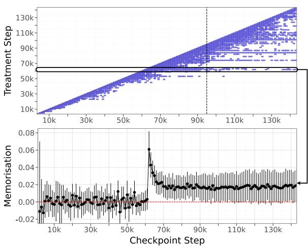
Because individual counterfactual outcomes cannot be observed, the method focuses on an average treatment effect over all examples treated at timestep $g$g:

The collection of values $\tau_{g,c}$τg,c​ across treatment timesteps $g$g and checkpoint timesteps $c$c forms a memorization profile. Each row of this profile represents the memorization path for a batch of examples introduced at timestep $g$g. There is no memorization for checkpoints before exposure, so $\tau_{g,c}=0$τg,c​=0 when $c<g$c<g. The effect is called instantaneous memorization when $c=g$c=g, persistent memorization when $c>g$c>g, and residual memorization when $c=T$c=T.

For estimation, the authors first observe the factual outcome for examples in the training batch $B_g$Bg​. They define the batch-average observed performance at checkpoint $c$c as:

The first term in the causal estimand can be directly estimated with this quantity. The second term,

is counterfactual because examples in $B_g$Bg​ were in fact used for training. To address this issue, the authors derive two estimators that replace the unobserved counterfactual with observable proxy outcomes.

The first is the difference estimator. Under the assumption that training and validation examples are independently and identically distributed and that examples are randomly assigned to batches or validation sets, the expected performance on untreated validation examples approximates the expected counterfactual performance of treated examples. The corresponding estimator is:

where $B_\infty$B∞​ denotes a held-out validation set. This estimator uses only observed outcomes at checkpoint $c$c. It compares the average performance of a trained batch with the average performance of untrained validation examples. The method requires strong distributional matching between training and validation sets, and its variance can remain high because the batch mean $\overline{Y}_c(g)$Yc​(g) is restricted to examples in $B_g$Bg​.

The main estimation procedure uses a difference-in-differences design. This approach uses the time dimension to identify the treatment effect by comparing how performance changes over checkpoints for treated examples and untreated examples. It relies on parallel trends and no anticipation. Parallel trends means that, in the absence of training, the expected change in performance across checkpoints would be the same for treated and untreated examples:

No anticipation means that training at timestep $g$g cannot affect performance at any checkpoint $c<g$c<g:

Under these conditions, the target causal estimand can be rewritten using observable panel outcomes. The difference-in-differences estimand is:

In practice, the authors evaluate model performance for a subset of training batches and validation examples at the checkpoint immediately before treatment, $g-1$g−1, and at a later checkpoint $c$c. This creates a panel of observed outcomes, analogous to repeated measurements in causal inference. The difference-in-differences estimator is computed as:

This workflow uses only observed outcomes from a model checkpoint sequence. For each batch $B_g$Bg​, the method measures how much the model’s performance on that batch changes after the batch becomes available for training, while subtracting the background change observed on examples that remain untrained. This difference controls for general improvements that happen over time across the model, rather than improvements caused by exposure to specific training batches.

The authors also describe influence functions as an alternative instance-level approximation for estimating counterfactual memorization at the final checkpoint. Influence functions estimate how parameters would change if an example were removed from the training set, without retraining:

where $\mathrm{H}_{\boldsymbol{\theta}}$Hθ​ is the Hessian of the training loss evaluated at $\boldsymbol{\theta}_{T}$θT​. The estimated counterfactual performance is obtained by evaluating the example using the adjusted parameters:

The corresponding influence-function memorization estimate is:

This approach avoids repeated retraining and provides an instance-level estimate, but it depends on convexity, positive definiteness of the Hessian, and convergence assumptions that are generally weak for large language models. It also applies only at the final checkpoint, so it cannot characterize memorization dynamics across intermediate checkpoints.

Experiment

The experiments evaluate memorisation in Pythia language models ranging from 70M to 12B parameters using a subsampled panel of training instances measured across checkpoints with sequence-level log-likelihood. They find that instantaneous memorisation is stronger early in training and increases with model size, while persistent memorisation is weak or absent in small models and tends to plateau after a fixed number of steps. Residual memorisation is often statistically insignificant, though a recency effect appears near the end of training, and overall memorisation patterns across model sizes are broadly predictable.