One-sentence Summary

Google Research proposes modeling dense, long-term motion as spectral volumes in the Fourier domain, predicted by diffusion models trained on natural oscillatory trajectories extracted from real video, enabling still images to be converted into seamlessly looping videos or interactively animated via image-space modal bases.

Key Contributions

• A learned image-space prior for natural oscillatory scene motion is obtained from motion trajectories extracted from real videos of trees, flowers, candles, and clothing, and represents dense long-term motion as spectral volumes in the Fourier domain.

• A frequency-coordinated diffusion sampling model predicts a spectral volume from a single image and converts the predicted spectral volume into a motion texture spanning a video. Fourier-domain spectral volumes are used because they are well suited to generative motion prediction.

• Image-based rendering uses the predicted spectral volume to produce seamlessly looping videos, motion editing, and interactive dynamic images that respond to user-applied forces by interpreting spectral volumes as image-space modal bases.

Introduction

Natural scenes contain subtle oscillations, and reproducing such motion is important for visual content synthesis because viewers quickly notice missing or unrealistic movement. Existing generative video models often struggle with coherent long term motion, temporal texture drift, and physical plausibility, while image animation methods may require driving videos, user annotations, or limited motion representations, and many motion prediction methods focus on optical flow or recognition rather than trainable motion priors for synthesis. The authors address this by learning a generative prior over image space scene motion using a frequency domain representation called a spectral volume. They extract dense long range pixel motion trajectories from real videos, train a diffusion model to predict spectral volumes from a single image, and coordinate predictions across frequencies with shared attention. The resulting model can turn still images into animations, support seamless looping and motion editing, and enable interactive dynamic images by using learned motion as an image space modal basis.

Dataset

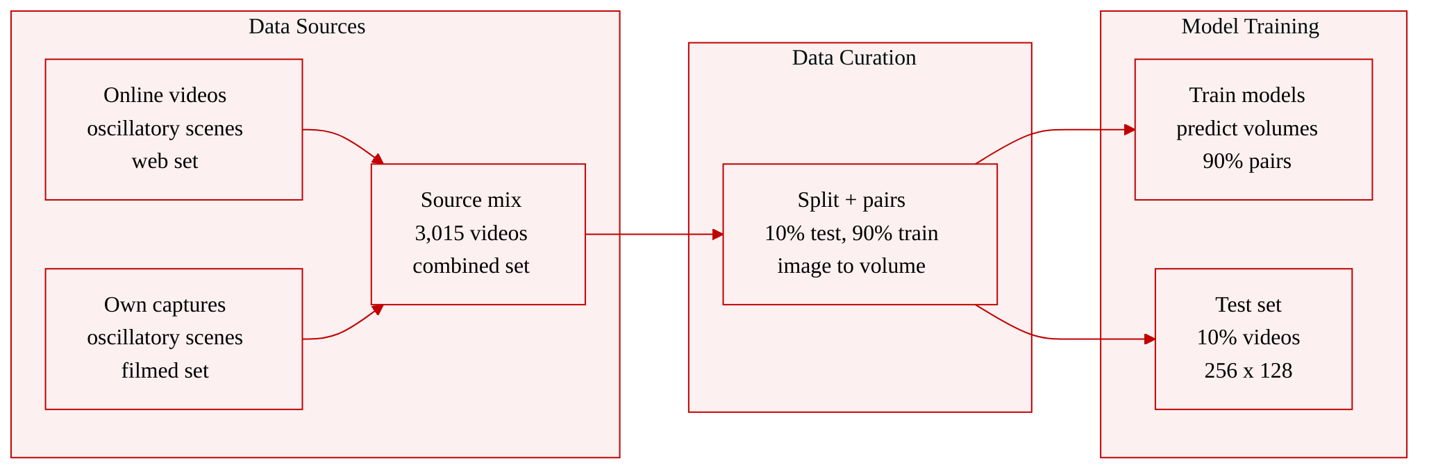
• The authors use a video dataset of 3,015 natural-scene videos showing oscillatory motions, collected from online sources and their own captures.

• The split is video-level: 10% of the videos are withheld for testing, and the remaining 90% are used for training.

• For supervision, the authors extract ground-truth motion trajectories with a coarse-to-fine optical-flow method between each selected starting frame and future frames.

• Training samples are constructed by taking every 10th video frame as the input image and computing corresponding ground-truth spectral volumes from motion trajectories over the following 149 frames.

• The resulting training pairs total more than 150K image-to-spectral-volume examples.

• For quantitative evaluation, the VAE and latent diffusion model are trained on images at 256 × 160 resolution; metric evaluation uses center-cropped frames at 256 × 128.

Method

The authors build a two-module image to video system. Given a single still image $I_0$I0​, the target is a generated sequence $\{\hat{I}_1, \hat{I}_2, \ldots, \hat{I}_T\}${I^1​,I^2​,…,I^T​} that shows quasi periodic motion such as swaying vegetation or flickering flames. The first module predicts a compact representation of future pixel motion, and the second module uses that motion to animate the input image. This separation lets the model reason about motion directly in the frequency domain while preserving the appearance of the original photograph.

At the level of motion representation, the authors do not predict a full sequence of dense displacement maps in the time domain. A motion texture is a sequence of 2D displacement fields $\mathcal{F} = \{F_t\}_{t=1}^T$F={Ft​}t=1T​, where each $F_t(\mathbf{p})$Ft​(p) maps a pixel $\mathbf{p}$p in $I_0$I0​ to its future location at time $t$t. Forward warping with such a field produces an incomplete warped frame,

Predicting all $T$T displacement fields directly would scale the output representation with video length, and independently predicted frames often drift over time. Instead, the authors represent per-pixel trajectories in the temporal Fourier domain as a spectral volume

A spectral volume is therefore a frequency space encoding of pixel motion. The time-domain motion texture is recovered by inverse Fourier transform,

Because many natural oscillations are dominated by low frequencies, the model does not need to represent the entire temporal spectrum. The authors keep a small number $K$K of frequency components, with $K \ll T$K≪T, and in practice use the first $K=16$K=16 terms. This choice is motivated by the observed decay of motion energy as frequency increases. The spectral distribution and the normalization strategy used to make these coefficients suitable for diffusion training are shown in the figure below:

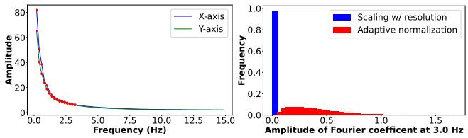
The figure shows why frequency-aware normalization matters. Raw spectral coefficients can have large amplitudes at low frequencies and rapidly decaying magnitudes at higher frequencies. If all coefficients are scaled only by image size, high-frequency terms collapse toward zero, and small denoising errors become large after inverse Fourier transform and denormalization. To avoid this, the authors compute a per-frequency scaling factor $s_{f_j}$sfj​​ as the 95th percentile of coefficient magnitudes in the training data, then apply a signed square-root transformation,

This keeps each frequency band within a more stable numeric range while preserving relative variation within the band.

For motion prediction, the authors leverage a latent diffusion model rather than a pixel-space diffusion model. The system first encodes a spectral volume into latent features through a variational autoencoder encoder, adds noise according to a diffusion schedule, and trains a U-Net denoiser to estimate the injected noise. During training, the model is conditioned on the first frame $I_0$I0​, so the learned motion prior is image dependent. The standard latent diffusion training objective is

where $z^n$zn is the noisy latent representation of a real spectral volume, $n$n is the diffusion time step, and $c$c is the conditioning signal. At inference time, denoising starts from Gaussian noise, and the denoised latent features are decoded back into a predicted spectral volume $\boldsymbol{S}$S.

The motion prediction architecture is shown in the figure below:

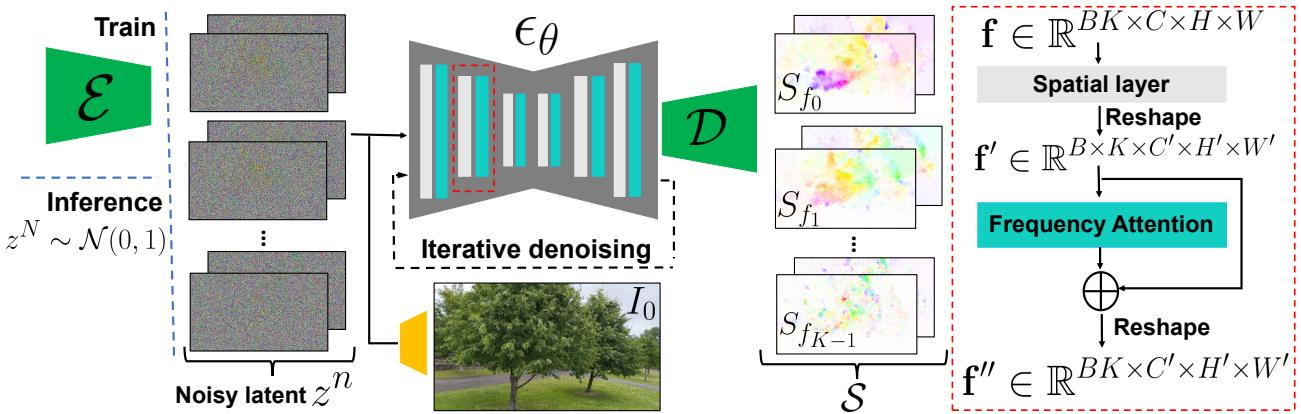
A key design question is how to output multiple frequency bands without producing either overly smooth or temporally inconsistent motion. A straightforward solution would be to train one U-Net to output a tensor with $4K$4K channels, where each frequency contributes complex Fourier coefficients for the horizontal and vertical displacement components. However, generating many channels in one shot can lead to oversmoothed and inaccurate motion. Another option is to predict each frequency slice independently using a frequency embedding, but this can break correlations across frequencies and produce unrealistic trajectories.

To balance expressiveness and coherence, the authors use a frequency-coordinated denoising module. They first train a base diffusion model to denoise a single 4-channel frequency slice, injecting a frequency embedding alongside the time-step embedding. This base model is then frozen, and attention layers are inserted between the spatial layers of the U-Net. These attention layers operate across the $K$K frequency bands. In their intermediate feature tensor, the $B \cdot K$B⋅K samples corresponding to different frequencies are first treated as independent spatial batches,

and then reshaped so that attention can be applied along the frequency axis,

After frequency attention, the features are reshaped back into the spatial batch layout. In this way, each frequency slice is denoised jointly with the others, allowing the model to enforce coherent spectral structure across low and higher motion modes. The denoised latents are finally decoded into the full spectral volume.

Once the spectral volume is predicted, it is transformed back into a motion texture through inverse temporal Fourier transform at each pixel. The rendering module then uses this motion texture to forward-warp the input image into future frames. Because forward warping creates holes where no source pixels land and also causes multiple source pixels to collide at the same destination, the authors do not rely on simple pixel splatting. Instead, they use a deep image-based rendering architecture with a feature pyramid softmax splatting operation.

The rendering pipeline is shown in the figure below:

The renderer begins by encoding $I_0$I0​ through a feature extractor network into multiple feature scales. For each scale, the motion field $F_t$Ft​ is resized and scaled to match the feature resolution. The authors also compute motion-derived weights,

which estimate the average motion magnitude at each pixel. This provides a depth-like proxy in the single-view setting: pixels with large motion are treated as foreground elements that should dominate their destination locations, while static or slowly moving pixels are treated as background. Softmax splatting then projects the multi-scale features to the target frame using $F_t$Ft​ and $W$W.

The warped multi-scale features are injected into a synthesis network that fills in missing content and refines the forward-warped image to produce the final rendered frame $\hat{I}_t$I^t​. The feature extractor and synthesis network are trained jointly on video pairs. For a pair $(I_0, I_t)$(I0​,It​), the network is trained to warp the encoded features from $I_0$I0​ using the ground-truth flow field from $I_0$I0​ to $I_t$It​, and predictions are supervised against $I_t$It​ with a VGG perceptual loss. Since the renderer depends on projected features, its output is naturally sensitive to thin moving objects, large displacements, and regions that require substantial new content. These failure cases are visible below:

The frequency-domain motion representation also supports additional inference-time controls. For seamless looping, the authors add a motion self-guidance signal to the denoising process. At denoising step $n$n, the predicted displacement fields $F_1^n$F1n​ and $F_T^n$FTn​ are compared in both position and spatial gradient, and the resulting guidance term encourages start and end states to match:

where

Here $w$w controls classifier-free guidance and $u$u controls the strength of the looping guidance. This lets a model trained on ordinary non-looping clips generate videos that satisfy loop constraints without changing the learned motion prior.

The same spectral volume can also be used for interactive dynamics. The frequency slices $S_{f_j}$Sfj​​ can act as image-space motion modes, and a physical response can be generated by modulating these modes with time-varying modal coordinates $\mathbf{q}_{f_j}(t)$qfj​​(t),

The modal coordinates can be simulated with a decoupled mass spring damper system in modal space, allowing a user-defined force to drive oscillation from a single still image. This turns the learned spectral volume from a passive motion predictor into an interpretable motion basis for downstream animation control.

Experiment

The experiments evaluate spectral-volume animation on a collected oscillatory video dataset, comparing against single-image animation, video prediction, and large video-diffusion baselines using image and video quality metrics, temporal stability analysis, and qualitative comparisons. The results show that the frequency-coordinated diffusion model produces more realistic and temporally coherent videos without the degradation over time seen in prior methods. Ablations and a user study further validate the importance of the key model components and demonstrate strong preference over large video models, while the discussion notes limitations for non-oscillatory or high-frequency motion.

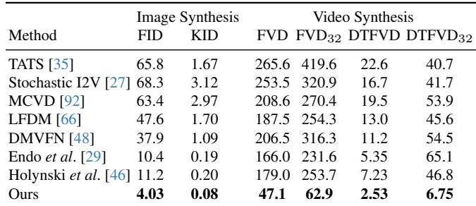
Quantitative test-set comparisons indicate that the proposed single-image animation method outperforms prior baselines on both image and video synthesis metrics. The improvement is especially pronounced for video distances such as FVD and DT-FVD, indicating more realistic and temporally coherent animations. The stability of quality over time is attributed to the global spectral volume representation. The method improves both image synthesis and video synthesis over prior single-image animation baselines. The larger reductions in FVD and DT-FVD point to better realism and temporal coherence. The global spectral volume representation helps maintain video quality over time.

The ablation results show that using more frequency bands generally improves video synthesis quality, with larger gains at lower band counts and more limited improvements beyond 16 bands. Removing adaptive normalization or the frequency coordinated denoising module leads to worse image and video synthesis quality than the full configuration. Video synthesis quality improves as frequency bands increase, but the benefit becomes marginal after 16 bands. Removing adaptive normalization or independent frequency prediction yields poorer video metrics than the full model.

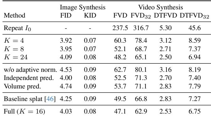
Quantitative test-set comparisons show that the proposed single-image animation method outperforms prior baselines in both image and video synthesis, with particularly strong gains in realism and temporal coherence. The ablation study indicates that increasing frequency bands generally improves video quality, although benefits plateau after 16 bands, and that adaptive normalization and frequency coordinated denoising are important for preserving image and video fidelity. Overall, the global spectral volume representation and the full model contribute to more stable, temporally coherent animations.